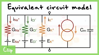
Electrical Circuit Model of the Plasma Membrane
A comprehensive guide to understanding the cell membrane as an electrical circuit, featuring interactive simulations, mathematical derivations, and Python code.
Learning Objectives
- •Model the plasma membrane as a parallel RC circuit with ion-specific conductances
- •Derive the Thévenin equivalent circuit and understand its physical meaning
- •Apply Kirchhoff's laws to calculate membrane potential and ionic currents
- •Understand the Hodgkin-Huxley model and its Nobel Prize-winning implications
- •Implement numerical simulations of action potentials using Python
⚡Interactive Membrane Circuit Diagram
Channel Conductances
E_Na = +61 mV • I = -145.72 µA/cm²
E_K = -89 mV • I = 154.05 µA/cm²
E_Cl = -70 mV • I = -4.42 µA/cm²
E_Leak = -70 mV • I = -4.42 µA/cm²
Calculated Values
Thévenin Equivalent Circuit Derivation
The complex membrane circuit with multiple ion channels can be simplified to a single voltage source (Vth) in series with a single resistance (Rth). This Thévenin equivalent captures the essential electrical behavior of the membrane.
Step-by-Step Derivation
Step 1: Apply Kirchhoff's Current Law
At steady state, all ionic currents sum to zero:
Step 2: Express Each Current Using Ohm's Law
Step 3: Substitute and Solve for $V_m$
Collecting terms:
Step 4: Final Thévenin Voltage
This is the Goldman-Hodgkin-Katz equation!
Step 5: Thévenin Resistance
Numerical Example: Resting Neuron
Given Values (typical neuron)
g_total = 1 + 36 + 0.3 + 0.3 = 37.6 mS/cm²
V_th = (1×61 + 36×(-89) + 0.3×(-70) + 0.3×(-70)) / 37.6
V_th = (61 - 3204 - 21 - 21) / 37.6
V_th = -84.7 mV
R_th = 1000/37.6 = 26.6 Ω·cm²
Physical Interpretation
The resting potential (-70 mV) is close to E_K (-89 mV) because K⁺ conductance dominates at rest (36 out of 37.6 mS/cm²). The small Na⁺ conductance pulls V_m slightly positive from E_K.
Circuit Schematic Representations
Full Membrane Circuit
     EXTRACELLULAR (0 mV reference)
     ════════════════════════════════════════════════════════════
          │          │          │          │          │
          │         ┌┴┐        ┌┴┐        ┌┴┐        ┌┴┐
         ─┼─        │ │        │ │        │ │        │ │
        ──┼──       │ │gNa     │ │gK      │ │gCl     │ │gLeak
         ─┼─        │ │        │ │        │ │        │ │
          │         └┬┘        └┬┘        └┬┘        └┬┘
          │  Cm      │          │          │          │
          │          │          │          │          │
          │        ──┴──      ──┴──      ──┴──      ──┴──
          │       +│   │-    -│   │+    -│   │+    -│   │+
          │        │ E │      │ E │      │ E │      │ E │
          │        │Na │      │ K │      │Cl │      │ L │
          │        │+61│      │-89│      │-70│      │-70│
          │       ──┬──      ──┬──      ──┬──      ──┬──
          │          │          │          │          │
     ════════════════════════════════════════════════════════════
     INTRACELLULAR (Vm ≈ -70 mV)

     Cm = Membrane Capacitor (1 µF/cm²)
     gX = Ion Channel Conductance (variable resistor)
     EX = Nernst Equilibrium Potential (battery/EMF)
Thévenin Equivalent
     EXTRACELLULAR (0 mV)
     ═══════════════════════════════
               │
               │
              ┌┴┐
              │ │  Rth = 1/gtotal
              │ │      = 26.6 Ω·cm²
              │ │
              └┬┘
               │
             ──┴──
            +│   │-
             │Vth│  Vth = ΣgiEi/Σgi
             │   │      = -70 mV
            ──┬──
               │
               │
     ═══════════════════════════════
     INTRACELLULAR (Vm)


     ┌─────────────────────────────┐
     │  Time Constant:             │
     │  τ = Rth × Cm               │
     │    = 26.6 × 1 µF            │
     │    = 26.6 ms                │
     └─────────────────────────────┘
Complete Circuit with Na⁺/K⁺-ATPase Pump
     EXTRACELLULAR
     ══════════════════════════════════════════════════════════════════════════════
          │          │          │          │          │              │
          │         ┌┴┐        ┌┴┐        ┌┴┐        ┌┴┐            │
         ─┼─        │ │        │ │        │ │        │ │         ┌──┴──┐
        ──┼──       │ │gNa     │ │gK      │ │gCl     │ │gL       │PUMP │ 3Na⁺ OUT
         ─┼─        │ │        │ │        │ │        │ │         │     │──────►
          │         └┬┘        └┬┘        └┬┘        └┬┘         │ ATP │
          │  Cm      │          │          │          │          │     │ 2K⁺ IN
          │          │          │          │          │          │     │◄──────
          │        ──┴──      ──┴──      ──┴──      ──┴──        └──┬──┘
          │       +│   │-    -│   │+    -│   │+    -│   │+          │
          │        │ENa│      │ EK│      │ECl│      │ EL│          ─┼─  Current
          │        │+61│      │-89│      │-70│      │-70│         ──┼── Source
          │       ──┬──      ──┬──      ──┬──      ──┬──          ─┼─  (Ipump)
          │          │          │          │          │              │
     ══════════════════════════════════════════════════════════════════════════════
     INTRACELLULAR (Vm)

     Na⁺/K⁺-ATPase: Electrogenic pump that maintains ion gradients
     • Exports 3 Na⁺ ions → Creates outward current
     • Imports 2 K⁺ ions  → Net charge movement = hyperpolarizing
     • Ipump ≈ 0.5-1.0 µA/cm² (contributes ~5 mV to resting potential)
Action Potential Waveform & Conductance Changes
    Vm (mV)
    +40 ┤                    ╭─╮
        │                   ╱   ╲
    +20 ┤                  ╱     ╲
        │                 ╱       ╲
      0 ┤                ╱         ╲
        │               ╱           ╲
    -20 ┤              ╱             ╲
        │             ╱               ╲
    -40 ┤            ╱                 ╲
        │           ╱                   ╲
    -55 ┤─ ─ ─ ─ ─╱─Threshold─ ─ ─ ─ ─ ─╲─ ─ ─ ─ ─ ─ ─ ─ ─
        │        ╱                       ╲
    -70 ┼───────╱                         ╲───────────────── Resting
        │      ↑                           ╲_____╱
    -90 ┤    Stimulus                    Undershoot (AHP)
        └────┴────┴────┴────┴────┴────┴────┴────┴────┴────► Time (ms)
             0    1    2    3    4    5    6    7    8

    Conductances:
    ━━━━━━━━━━━━━━━━━━━━━━━━━━━━━━━━━━━━━━━━━━━━━━━━━━━━━━━━━━━━━━━━━━
    gNa         ┌────╮                      (Fast activation, fast inactivation)
    (red)  ─────┘    ╰─────────────────────────────────────────────────
    ━━━━━━━━━━━━━━━━━━━━━━━━━━━━━━━━━━━━━━━━━━━━━━━━━━━━━━━━━━━━━━━━━━
    gK              ┌──────────────╮        (Slow activation, no inactivation)
    (green) ────────┘              ╰───────────────────────────────────
    ━━━━━━━━━━━━━━━━━━━━━━━━━━━━━━━━━━━━━━━━━━━━━━━━━━━━━━━━━━━━━━━━━━

    PHASES:
    1. REST:       gK >> gNa  →  Vm near EK (-89 mV), but modified by other channels
    2. RISING:     gNa >> gK  →  Vm rushes toward ENa (+61 mV)
    3. PEAK:       Na⁺ inactivation begins (h gate closes)
    4. FALLING:    gK increases, gNa decreases → Vm returns toward EK
    5. UNDERSHOOT: gK still elevated → Vm briefly more negative than rest
Conductance State Comparison
① Resting State
gK dominates → Vm ≈ −70 mV
gNa ▓░░░░░░░░░░░░░░░░░░░  1 mS/cm²
gK  ▓▓▓▓▓▓▓▓▓▓▓▓▓▓▓▓▓▓▓▓  36 mS/cm²
gCl ▓▓░░░░░░░░░░░░░░░░░░  0.3 mS/cm²
Vm = (1×61 + 36×(−89) + 0.3×(−70)) / 37.3 ≈ −70 mV
② Depolarized (AP Peak)
gNa dominates → Vm ≈ +40 mV
gNa ▓▓▓▓▓▓▓▓▓▓▓▓▓▓▓▓▓▓▓▓  120 mS/cm²
gK  ▓▓▓▓▓▓▓▓▓▓▓▓▓▓▓▓▓▓▓▓  36 mS/cm²
gCl ▓▓░░░░░░░░░░░░░░░░░░  0.3 mS/cm²
Vm = (120×61 + 36×(−89)) / 156 ≈ +26 mV
③ Repolarizing (AHP)
gK elevated → Vm → −89 mV
gNa ▓░░░░░░░░░░░░░░░░░░░  ~0 mS/cm²
gK  ▓▓▓▓▓▓▓▓▓▓▓▓▓▓▓▓▓▓▓▓  72 mS/cm²
gCl ▓▓░░░░░░░░░░░░░░░░░░  0.3 mS/cm²
Vm ≈ EK = −89 mV (undershoot)
Complete Circuit Theory
Batteries (E_ion)
Each ion's Nernst potential acts as an EMF source. The "battery" drives ions toward equilibrium.
E_Na = +61 mV (pulls positive)
E_K = -89 mV (pulls negative)
Resistors (g_ion)
Conductance (g = 1/R) represents how easily ions flow. Higher g means more current.
g_K at rest ≈ 36 mS/cm²
g_Na at rest ≈ 1 mS/cm²
Capacitor (C_m)
The lipid bilayer acts as a dielectric, storing charge and slowing voltage changes.
C_m ≈ 1 µF/cm²
d ≈ 7-8 nm thickness
Current Source (Pump)
The Na⁺/K⁺-ATPase is an electrogenic pump, contributing a small outward current.
3 Na⁺ out / 2 K⁺ in
Contributes ~-10 mV
Key Equations
Nernst Equation
At 37°C: $E_X = \frac{61.5}{z} \log_{10} \frac{[X]_o}{[X]_i}$ mV
Ohm's Law for Ion Channels
Current flows when $V_m \neq E_{\text{ion}}$ (driving force exists)
Kirchhoff's Current Law
At steady state: $I_{\text{Na}} + I_{\text{K}} + I_{\text{Cl}} + I_{\text{Leak}} = 0$
Goldman-Hodgkin-Katz Equation
Weighted average of equilibrium potentials, weighted by conductances
RC Time Constant
$\tau \approx 2\text{-}5$ ms for neurons. Time for $V_m$ to reach 63% of final value.
Membrane Capacitor Equation
Capacitive current only flows during voltage changes
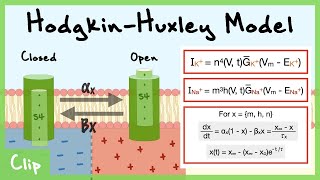
Hodgkin-Huxley Gating Variables
The Nobel Prize-winning Hodgkin-Huxley model (1952) introduced voltage-dependent gating variables that describe how ion channel conductances change during an action potential.
Na⁺ Channel
m: activation gate (fast)
h: inactivation gate (slow)
K⁺ Channel
n: activation gate (slow)
Delayed rectifier current
Gating Kinetics
$\alpha$ and $\beta$ are voltage-dependent rate constants
Complete Hodgkin-Huxley Equation
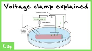
Experimental Measurement Techniques
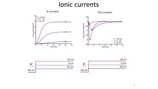
Voltage Clamp
Developed by Cole (1949) and perfected by Hodgkin & Huxley (1952). The technique uses negative feedback to hold V_m constant while measuring the current required.
- • Measures ionic currents at fixed potentials
- • Separates Na⁺ and K⁺ currents pharmacologically
- • Used to determine g-V relationships
Patch Clamp
Invented by Neher & Sakmann (1976, Nobel Prize 1991). Records currents through individual ion channels with pA resolution.
- • Cell-attached, whole-cell, inside-out, outside-out
- • Single channel conductances: 10-50 pS typical
- • Reveals channel gating kinetics
Nobel Prize Recognition
• 1963: Hodgkin & Huxley (ionic mechanisms of action potentials)
• 1991: Neher & Sakmann (patch clamp technique)
Key Circuit Insights
The Weighted Average Principle
The plasma membrane circuit reveals that the resting potential (−70 mV) is simply a weighted average of all open ion pathways:
Na⁺ at +61 mV
Pulls membrane positive (depolarizing). Opening Na⁺ channels shifts V_m toward +61 mV.
K⁺ at −89 mV
Pulls membrane negative (hyperpolarizing). K⁺ dominates at rest because g_K >> g_Na.
Demystifying the Action Potential
The action potential requires no mystical properties—just parallel resistors and batteries!
- 1Depolarization: Voltage-gated Na⁺ channels open, increasing g_Na from 1 to ~120 mS/cm². V_m shifts from −70 toward +61 mV.
- 2Peak: V_m reaches ~+40 mV (not quite E_Na because g_K is still present). Na⁺ channels begin inactivating (h → 0).
- 3Repolarization: K⁺ channels open (delayed), increasing g_K. V_m returns toward −89 mV as K⁺ conductance dominates.
- 4Afterhyperpolarization: K⁺ channels remain open briefly, pushing V_m below resting (−80 to −90 mV) before returning to rest.
"Opening more Na⁺ channels repels the potential away from E_K toward E_Na. This beautifully explains action potential generation without invoking any mystical properties—just parallel resistors and batteries!"
Video Lectures
Comprehensive video series covering membrane electrophysiology, circuit models, and the Hodgkin-Huxley framework.
Featured: Hodgkin-Huxley Model Explained
Electrophysiology Basics
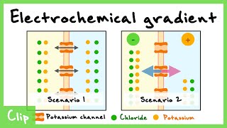
Nernst Equation And The Electrochemical Gradient Explained
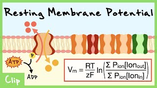
Goldman Equation And The Resting Membrane Potential Explained
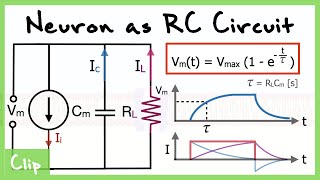
Neuron As RC Circuit Explained And Analysis of the Time Constant Tau
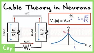
Cable Theory Model of the Neuron And Analysis Of The Space Constant Lambda
Equivalent Circuit Model Of The Neuron Explained (Capacitance, Resistance, Driving force)
Voltage Clamp Explained (Tetrodotoxin And Tetraethylammonium)

Action Potential Propagation And The Refractory Period Explained

Myelin And Axon Diameter Effect On Action Potential Conduction Velocity

Patch Clamp Explained (Cell-Attached, Whole Cell, Inside Out, Outside Out)
Hodgkin-Huxley Model of Voltage-Gated Channels Explained (Gating Variables n, m, h)
Python Simulation Of The Hodgkin-Huxley Model
MIT 9.40: Introduction to Neural Computation
Complete 20-lecture course covering biophysics to neural networks
Lecture 4: Hodgkin-Huxley Model Part 1
MIT 1: Course Overview and Ionic Currents
MIT 2: Resistor Capacitor Circuit and Nernst Potential
MIT 3: Resistor Capacitor Neuron Model
MIT 4: Hodgkin-Huxley Model Part 1
MIT 5: Hodgkin-Huxley Model Part 2
MIT 6: Dendrites
MIT 7: Synapses
MIT 8: Spike Trains
MIT 9: Receptive Fields
MIT 10: Time Series
MIT 11: Spectral Analysis Part 1
MIT 12: Spectral Analysis Part 2
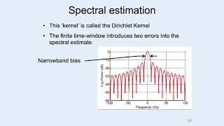
MIT 13: Spectral Analysis Part 3
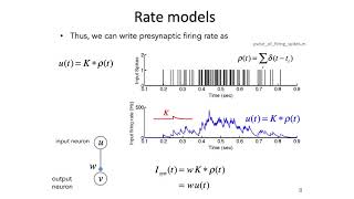
MIT 14: Rate Models and Perceptrons

MIT 15: Matrix Operations
MIT 16: Basis Sets

MIT 17: Principal Components Analysis
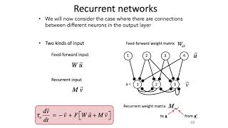
MIT 18: Recurrent Networks
MIT 19: Neural Integrators
MIT 20: Hopfield Networks
Simulation Code
Run simulations directly in your browser using Pyodide (Python in WebAssembly), or download to run locally.
Simple Membrane Potential Calculator
Calculate membrane potential using the parallel conductance model. Click 'Run in Browser' to execute.
# Simple Membrane Potential Calculator
# Using the parallel conductance model
import numpy as np
def calculate_membrane_potential(conductances, potentials, I_pump=0):
"""
Calculate membrane potential using the Goldman-Hodgkin-Katz equation.
Parameters:
-----------
conductances : dict
Dictionary of ion conductances in mS/cm²
e.g., {'Na': 1, 'K': 36, 'Cl': 0.3, 'Leak': 0.3}
potentials : dict
Dictionary of equilibrium potentials in mV
e.g., {'Na': 61, 'K': -89, 'Cl': -70, 'Leak': -70}
I_pump : float
Pump current in µA/cm² (default 0)
Returns:
--------
dict : Contains Vm, Rth, tau, and individual currents
"""
# Calculate total conductance
g_total = sum(conductances.values())
# Calculate membrane potential (weighted average)
numerator = sum(conductances[ion] * potentials[ion]
for ion in conductances) - I_pump
Vm = numerator / g_total
# Calculate individual currents
currents = {ion: conductances[ion] * (Vm - potentials[ion])
for ion in conductances}
# Thévenin equivalent
Rth = 1000 / g_total # Ω·cm²
# Time constant (assuming Cm = 1 µF/cm²)
Cm = 1.0
tau = Cm * Rth / 1000 # ms
return {
'Vm': Vm,
'g_total': g_total,
'Rth': Rth,
'tau': tau,
'currents': currents
}
# Example: Resting neuron
conductances = {'Na': 1, 'K': 36, 'Cl': 0.3, 'Leak': 0.3}
potentials = {'Na': 61, 'K': -89, 'Cl': -70, 'Leak': -70}
result = calculate_membrane_potential(conductances, potentials)
print("=== Resting Membrane Analysis ===")
print(f"Membrane Potential: {result['Vm']:.2f} mV")
print(f"Total Conductance: {result['g_total']:.2f} mS/cm²")
print(f"Thévenin Resistance: {result['Rth']:.2f} Ω·cm²")
print(f"Time Constant: {result['tau']:.2f} ms")
print("\nIndividual Currents (µA/cm²):")
for ion, current in result['currents'].items():
print(f" I_{ion}: {current:.3f}")
# Example: Action potential peak (high Na+ conductance)
print("\n=== Action Potential Peak ===")
conductances_ap = {'Na': 120, 'K': 36, 'Cl': 0.3, 'Leak': 0.3}
result_ap = calculate_membrane_potential(conductances_ap, potentials)
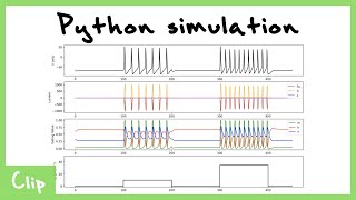
print(f"Membrane Potential: {result_ap['Vm']:.2f} mV")Complete Hodgkin-Huxley Simulation
Full implementation with RK4 integration and gating kinetics. Runs in browser without matplotlib plotting.
import numpy as np
import matplotlib.pyplot as plt
def odeint(f, y0, t, args=(), full_output=False):
    y0 = np.array(y0, dtype=float); t = np.asarray(t, dtype=float)
    n = len(y0); ys = np.zeros((len(t), n)); ys[0] = y0; y = y0.copy()
    for i in range(1, len(t)):
        h = t[i] - t[i-1]
        k1 = np.array(f(y, t[i-1], *args), dtype=float)
        k2 = np.array(f(y+.5*h*k1, t[i-1]+.5*h, *args), dtype=float)
        k3 = np.array(f(y+.5*h*k2, t[i-1]+.5*h, *args), dtype=float)
        k4 = np.array(f(y+h*k3, t[i], *args), dtype=float)
        y = y + (h/6)*(k1+2*k2+2*k3+k4); ys[i] = y
    return ys

# Hodgkin-Huxley Model Parameters (Giant Squid Axon)
C_m = 1.0      # Membrane capacitance (µF/cm²)
g_Na_max = 120.0  # Max Na+ conductance (mS/cm²)
g_K_max = 36.0    # Max K+ conductance (mS/cm²)
g_L = 0.3         # Leak conductance (mS/cm²)
E_Na = 50.0       # Na+ reversal potential (mV)
E_K = -77.0       # K+ reversal potential (mV)
E_L = -54.4       # Leak reversal potential (mV)

# Rate constants (alpha and beta functions)
def alpha_m(V): return 0.1 * (V + 40) / (1 - np.exp(-(V + 40) / 10))
def beta_m(V):  return 4.0 * np.exp(-(V + 65) / 18)
def alpha_h(V): return 0.07 * np.exp(-(V + 65) / 20)
def beta_h(V):  return 1.0 / (1 + np.exp(-(V + 35) / 10))
def alpha_n(V): return 0.01 * (V + 55) / (1 - np.exp(-(V + 55) / 10))
def beta_n(V):  return 0.125 * np.exp(-(V + 65) / 80)

# Hodgkin-Huxley differential equations
def hodgkin_huxley(y, t, I_ext):
    V, m, h, n = y

    # Ionic currents
    I_Na = g_Na_max * m**3 * h * (V - E_Na)
    I_K = g_K_max * n**4 * (V - E_K)
    I_L = g_L * (V - E_L)

    # Membrane potential derivative
    dVdt = (I_ext - I_Na - I_K - I_L) / C_m

    # Gating variable derivatives
    dmdt = alpha_m(V) * (1 - m) - beta_m(V) * m
    dhdt = alpha_h(V) * (1 - h) - beta_h(V) * h
    dndt = alpha_n(V) * (1 - n) - beta_n(V) * n

    return [dVdt, dmdt, dhdt, dndt]

# Simulation parameters
T = 50.0      # Total time (ms)
dt = 0.01     # Time step (ms)
t = np.arange(0, T, dt)

# Initial conditions (resting state)
V0 = -65.0    # Resting potential (mV)
m0 = alpha_m(V0) / (alpha_m(V0) + beta_m(V0))
h0 = alpha_h(V0) / (alpha_h(V0) + beta_h(V0))
n0 = alpha_n(V0) / (alpha_n(V0) + beta_n(V0))
y0 = [V0, m0, h0, n0]

# External current stimulus
def I_stim(t):
    return 10.0 if 10 < t < 40 else 0  # 10 µA/cm² from t=10-40 ms

# Solve using RK4 (via odeint)
I_ext_array = [I_stim(ti) for ti in t]
solution = odeint(lambda y, ti: hodgkin_huxley(y, ti, I_stim(ti)), y0, t)

# Extract results
V = solution[:, 0]
m = solution[:, 1]
h = solution[:, 2]
n = solution[:, 3]

# Calculate conductances
g_Na = g_Na_max * m**3 * h
g_K = g_K_max * n**4

# Plot results
fig, axes = plt.subplots(3, 1, figsize=(10, 8), sharex=True)

axes[0].plot(t, V, 'b-', linewidth=1)
axes[0].set_ylabel('V_m (mV)')
axes[0].set_title('Hodgkin-Huxley Action Potential Simulation')
axes[0].axhline(-65, color='gray', linestyle='--', alpha=0.5)

axes[1].plot(t, m, 'r-', label='m (Na activation)')
axes[1].plot(t, h, 'r--', label='h (Na inactivation)')
axes[1].plot(t, n, 'g-', label='n (K activation)')
axes[1].set_ylabel('Gating variables')
axes[1].legend()

axes[2].plot(t, g_Na, 'r-', label='g_Na')
axes[2].plot(t, g_K, 'g-', label='g_K')
axes[2].set_xlabel('Time (ms)')
axes[2].set_ylabel('Conductance (mS/cm²)')
axes[2].legend()

plt.tight_layout()
plt.savefig('hodgkin_huxley_simulation.png', dpi=150)
plt.show()
Fortran + Python: Hodgkin-Huxley Model with Visualization
PythonCompiles and runs a Fortran HH neuron simulation with RK4 integration, then plots membrane potential, gating variables, conductances, and ion currents
Click Run to execute the Python code
Code will be executed with Python 3 on the server
Validation Checklist for Debugging
Physical Checks
- ✓ Resting V_m between -60 and -80 mV
- ✓ AP peak near +40 mV (not exceeding E_Na)
- ✓ AP duration 1-2 ms (squid axon)
- ✓ Refractory period ~1-2 ms
- ✓ Currents sum to zero at steady state
Numerical Checks
- ✓ dt ≤ 0.01 ms for stability
- ✓ Gating variables remain in [0, 1]
- ✓ No NaN or Inf values
- ✓ Energy conservation (current balance)
- ✓ Compare with literature values
References & Further Reading
- • Hodgkin AL, Huxley AF (1952). A quantitative description of membrane current and its application to conduction and excitation in nerve. J Physiol 117:500-544.
- • Hille B (2001). Ion Channels of Excitable Membranes, 3rd ed. Sinauer Associates.
- • Johnston D, Wu SM (1995). Foundations of Cellular Neurophysiology. MIT Press.
- • Kandel ER et al. (2021). Principles of Neural Science, 6th ed. McGraw-Hill.
- • Cole KS (1949). Dynamic electrical characteristics of the squid axon membrane. Arch Sci Physiol 3:253-258.